Last Time
Last time we looked at depth first search and how it could be applied to a simple optimization problem, the pancake problem. We decomposed the pancake stacking problem into some components are very important if you want to apply heuristic search:
- A goal test
- States
- Actions to move between states
We then looked at how these and other domain properties mapped to elements of the depth first search algorithm:
- Goal tests to know when you’re done
- States to get to nodes in the tree
- Actions to build successor functions to expand the tree
- Heuristics to improve search performance
- Equivalence checks to avoid cyclic reasoning in the algorithm
We looked at a few implementations of depth first search in sequence, starting with a text book implementation. Each implementation we looked at ran into some difficulty in solving larger and larger pancake problems. The goal was to give you a look at the heart and soul of depth first search before we got lost in the weeds. We left things off by noting that our bounds computation is weak, and that we didn’t sort children during search.
Learning Goals
We saved those details for today; By improving the bounds computation and using some child ordering, we’re going to sort some comically large stacks of pancakes. We’ll start by examining how improved bounds computation and child ordering impact search performance. This will serve two purposes: we’re going to examine several meanings for the word heuristic, and we’re going to take a detailed look at how one evaluates search algorithms. Our discussion on search algorithm evaluation will also talk a bit about how to consume the output of search algorithms, assuming that you don’t just love search for search’s sake like I do. After all of that, we’re going to take a look at the generality of search techniques by tackling a new problem, tour planning, without changing the search strategy. This is going to work pretty well, but we’ll expose one or two new weaknesses in our depth first search implementation to look at next time.
More Pancakes
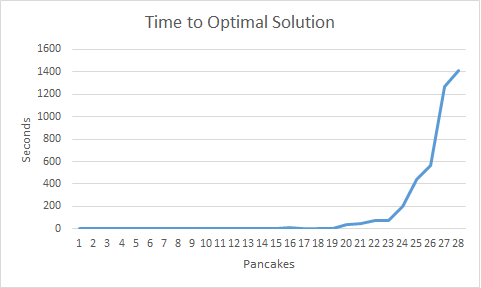
Last time, we ran out of patience when solving for stacks of six pancakes. That wasn’t very satisfying, either from a breakfast or an algorithm standpoint. Making a few modifications to the algorithm, we can get a performance curve like the one seen above. Small stacks, and even stacks too large for a single person to regularly consume, take fractions of a second to stack. As we get out to 30 pancakes in a stack, we’re seeing solving times in the tens of minutes, and if you wanted to plate hundreds of pancakes you would see solving times on the order of hours or days. Increasing the size of problems we can solve by an order of magnitude is generally seen as a really big thing in heuristic search. This is because the difficulty of problem solving grows very, very quickly as the size of the problem grows. Next, we’re going to look at how we got depth first search to scale up to these large problems and we’ll talk about what that whole “Time to Optimal Solution” thing in the plot means.
Heuristic Functions
Really, the only change we needed to make our approach skill was to improve the heuristics being used by depth first search. Heuristics, you may recall, tell us some information about the state. There are two major kinds of heuristics used in search: lower bounds and heuristic estimators. Lower bounds are, as the name implies, a lower bound on the cost of a solution passing through a given state. Heuristic estimators are anything else. These estimators serve different, but important purposes in search, as we will explore next.
Lower Bounds
Depth first search is often referred to as depth first branch and bound. Branching is the act of expanding a node to see which avenues of exploration can be considered from this point. Bounding is the process of cutting off these avenues of inquiry because they are not promising. In our last post, we were using little more than the cost of arriving at a given node as the cutoff point for bounding. However, with a lower bound heuristic, often referred to as an admissible heuristic, we can cut off a node much earlier:
- let g be the cost of arriving at a node, referenced by g(n)
- let h be a lower bound on a cost of a solution from a given node, referenced by h(n)
- then f is a lower bound on the total cost of a solution through a node, and is f(n) = g(n) + h(n)
Previously, we pruned out a node if the cost of reaching it was more than the incumbent. Now, we can discard a node if the lower bound on the cost of a solution through that node, f, is larger than the cost of the incumbent. In both cases we, or the search, are effectively saying “I will not consider this node because no solution better than the one I have can pass through it”. The addition of the heuristic function simply increases the number of nodes we don’t have to consider. The more nodes we can prune, the more work we can skip, and ultimately, the faster search goes.
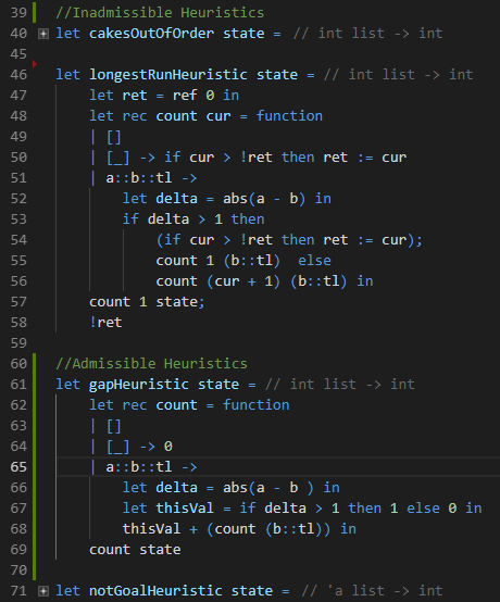
In our final implementation of our pancake solver, we used what is called the gap heuristic in the literature, shown in the figure above on lines 61-69. The gap heuristic is a count of the number of groups of pancakes in the stack that are already in sorted order or reverse sorted order. So, for example, in [1,2,3, 8,7,6,5,4 ], the gap heuristic produces two. [1,2,3] is a run and [8,7,6,5,4] is as well. The gap heuristic is, however just an approximation. The real cost of solving this state is 3 ( | is where the spatula goes) :
- [1,2,3,8,7,6,5,4 | ]
- [4,5,6,7,8 | ,3,2,1 ]
- [8, 7, 6, 5, 4, 3 , 2, 1 | ]
- [1,2,3,4,5,6,7,8]
Heuristic Estimators
The other heuristic shown above is not a lower bound. It’s another kind of heuristic entirely, one which suggests an ordering over children in the tree. Consider a 100 pancake problem, for a moment. There are 100 places to put the spatula in for any given state in that problem, which means that each node has a hundred children. When you consider the first child, before considering the second child, you have to consider the entire subtree beneath the first child. In the 100 pancake problem, this is a great many nodes; so many, in fact, that you may never see the second child of the root of the tree without very powerful pruning heuristics. Child ordering is really, really important.
While the gap heuristic computes the number of breaks in a stack of pancakes of decreasing size, this heuristic reports the size of the largest run of pancakes. This isn’t an admissible heuristic like the gap heuristic, but it does tell us something about the ‘goodness’ of a given state. All else being equal, we would expect states with a larger run of pancakes to be closer to being completed. By preferring to explore those children we believe to be better first, we’re more likely to find a good solution early, assuming our notion of ‘better’ is actually accurate. The faster we find a good solution, the more aggressively we can prune the tree, and the faster search proceeds over all.
Consuming Solutions, Pancakes
Depth First, Anytime
It should be clear from the above discussion of multiple solutions and pruning that depth first search produces not just one answer, but a steadily improving stream of answers. We typically call algorithms that behave this way ‘anytime algorithms’. They’re so named because they can be asked for their solution at ‘any time’ (though that solution may be “None!”). We can see this in the figures below. Both show the cost of the solutions found by depth first search as a function of time. The first plot shows solution improvements within the first minute, the second plot shows the improvement in solution quality out to about ten minutes.
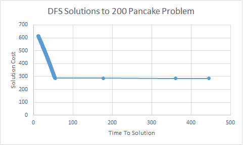
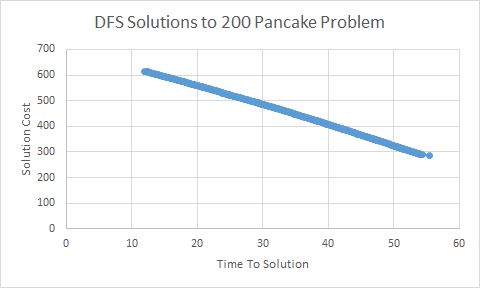
You can see in the plot with the shorter horizon that solutions improve steadily in the first minute. We find an initial solution of cost 600 and then steadily drive down the cost by about half over that minute. On the longer time line, you can see we don’t improve the solution much after this initial frenzied pace. We’re looking at both of the plots because that behavior is pretty typical of depth first search. Initially, the space of all solutions is very rich; we don’t have a good bound on solution cost and so many solutions are available to us. As we improve the solution cost, more and more solutions are discarded by pruning. Ultimately, no additional solutions remain because we have the optimal cost solution in hand. At that point, depth first search is just working on enumerating the entire space of all possible solutions to prove that the solution it already found is the best.
Heuristic Search Is A Means, Not an End
An important thing to note about anytime algorithms, and search in general, is that they are a means, not an end. Unless you’re doing your dissertation or just trying to get a handle on different types of algorithms, you’re typically employing search because there’s a problem that you want an answer to. The question becomes “well, I have a stream of solutions, when do I take a solution and run with it?” The answer to that question will depend almost entirely on your application. If you are computing an answer to a problem you encounter frequently, you probably want to wait as long as you can tolerate so that you can have the best solution you can find. Using a solution repeatedly allows for the cost of solving to be amortized out over the many applications of the answer. On the other hand, if you’re only going to encounter the problem once, you probably don’t want your solving costs to exceed the cost of executing the solution you find.
The Bran Tour
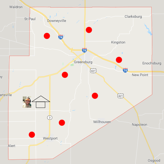
So, where did I get the batter for thousands upon thousands of pancakes? I went to the grocery store. Well, actually I went to a lot of grocery stores. For the number of pancakes we’re talking about, I probably went to every grocery store in the county. Again, time is of the essence. We’re trying to get these pancakes ready with minimal effort. Lets assume for a brief moment that there are only seven grocery stores in Decatur county and that I need to visit all of them to get the requisite amount of batter. That creates a problem like the one shown below:
Now, I need to visit every store, and then return home with a mountain of pancake mix. This is called a tour. I could compute one pretty cheaply by just going to the grocery store nearest to my house, and then the grocery store nearest to the grocery store I’m at, and so on before exhausting all stores and returning home. The tour resulting from this approach is shown below:
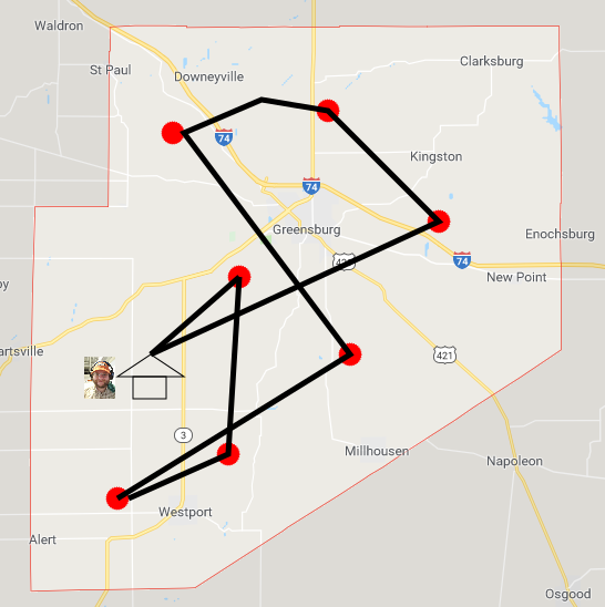
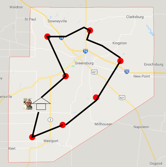
That kind of a solution is typically called a ‘greedy’ solution. It’s greedy in the sense that it greedily takes the ‘best’ action at a given avenue, in this case going to the nearest grocery store next. For most optimization problems, greedy algorithms don’t produce optimal solutions. You can see that the computed tour crosses itself in a few places. That’s inefficient. Search algorithms will let us compute the tour shown below, which is optimal:
The Travelling Salesman Problem
The problem we just presented is a very specific case of the widely studied travelling salesman problem, or TSP. The problem is generally stated as follows, given
- A set of locations L
- Distances between each pair of locations (l1,l2) in L
- A starting location l0
Find the shortest tour, starting at l0, passing through all points in L, and returning to l0. The TSP is pretty close to a lot of important industrial problems. Obviously it has applications in logistics, where you need to move product from a warehouse to a bunch of store fronts, then leave the vehicle back at the warehouse for tomorrow. Perhaps less obvious are applications of the TSP in manufacturing. Moving a welding arm between a number of spots to weld on a product and back to a starting position is exactly the TSP. Very large system integration (VLSI), the thing that lets us build integrated circuits out of transistors, is often cast as solving the TSP. Applications of the TSP tend to vary in the number of points that need visited and the way the cost of traveling between points is computed.
Representation Considerations
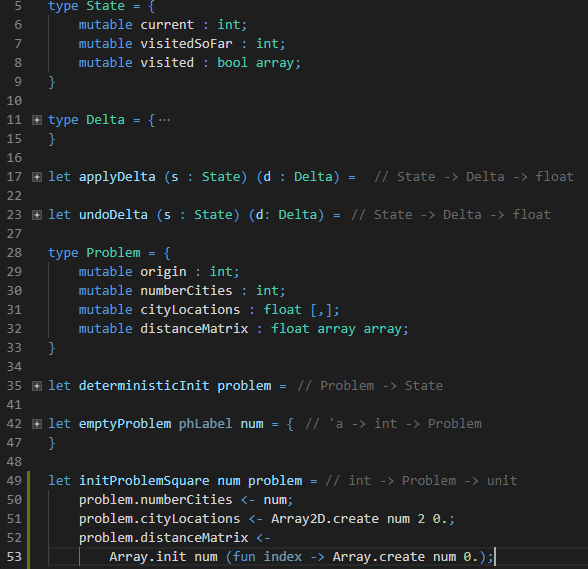
The first thing you need to do when tackling a new search problem is decide how you want to present it to the computer. The image above contains one of many possible ways of representing the TSP on a computer. It’s important to look at what we’ve chosen to say is a problem (lines 28-33) versus what we say is a state (lines 5-9). The problem contains a city of origin, a count of cities in the problem, an array of locations of those cities, and a distance matrix. The locations are just X,Y pairs on a 2D plane. For the grocery-store traveling problem we described above, that’s enough. In other applications, you may need three or more dimensions for the TSP.
States contain where the salesman currently is, a count of the cities they’ve visited so far, and a boolean array tracking which city indexes they’ve been to. It will be exceptionally important for us to know the distance between two cities in computing successor states of a given state. However, we don’t want to, nor can we afford to, store the cost of traveling between each pair of cities at every node. We’re splitting up the states and the problems with an eye towards memory consumption.
Conversely, we are storing data that could be computed on the fly: visitedSoFar ( line 7) and distanceMatrix (line 32). These are values we’ll want to access frequently, at least once per state. While the cost of computing distance between two points on a plane is small, if you intend to do anything millions or billions of times, costs add up quick. **We’re trading memory for speed, **and that’s a pretty common thing to do in heuristic searches of all stripes. We’ll see later that these algorithms are very resource hungry, so if you’re going to spend memory, you should do so judiciously.
Heuristics for the Problem
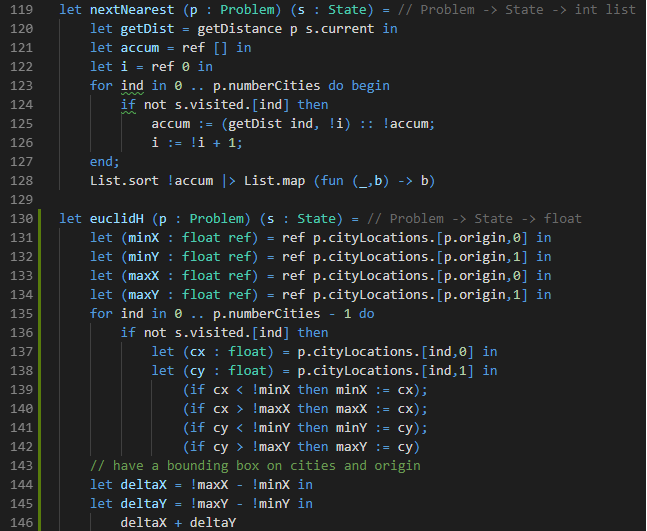
Recall from the pancake problem that there are (at least) two kinds of heuristics: those used for bounding the cost of a solution to the problem, and those used for ordering sibling nodes in the search tree. The image above shows two different heuristics for the TSP. nextNearest (lines 119-128) is a node ordering heuristic, which sorts unvisited cities by their proximity to the current city. This lines up exactly to the greedy solution strategy we discussed earlier. While the greedy solution won’t always find optimal solutions to the TSP, it does tend to find decent ones.
The second heuristic, on lines 130-146, is one of the bounding variety. In it, we compute a rectangle that encompasses all cities that have yet to be visited in the TSP as well as the city of origin. This says that “at the least, we must travel as far north south east and west as the furthest remaining city in each of those directions. Then we need to get back home. There are other more informative heuristics for the traveling salesman problem (e.g. the minimum spanning tree of all cities) that we’ll look at next time.
Replacing Pancakes with TSP in our Solver
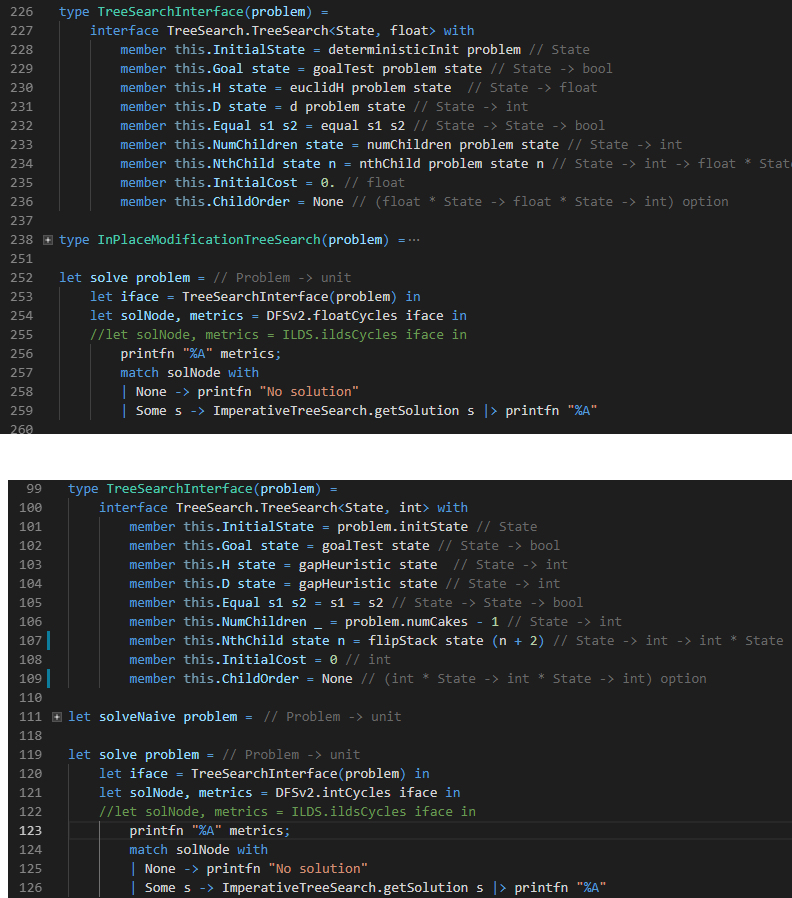
Above, we see calls for solving the traveling salesman problem as well as a call for solving the pancake problem. You can’t really tell which is which from the solve call; you have to look at how the heuristics and problem are being defined in the tree search interface. This is the primary benefit of heuristic search. It’s a general approach for problem solving. The search strategy is the same for solving the pancake problem as well as the TSP; we merely need change the underlying definition of problem.
Solving a ‘simple’ 100 City Problem
Solving a 100 city TSP isn’t too bad for the implementation show above. For the instance in question, we generate two solutions, a near-optimal solution a fraction of a second in. The optimal solution differs only slightly from the greedy solution, and is reported some ten minutes later. Considering the good performance of our TSP solver on a relatively small problem, maybe it can scale up to some truly ludicrous grocery store tours.
That Worked Well, How High Can We Scale?
100 grocery stores is nice, but that’s just not enough batter for the ridiculous number of pancakes we’d like to make. Let’s see how big of a problem we can tackle without changing our strategy:
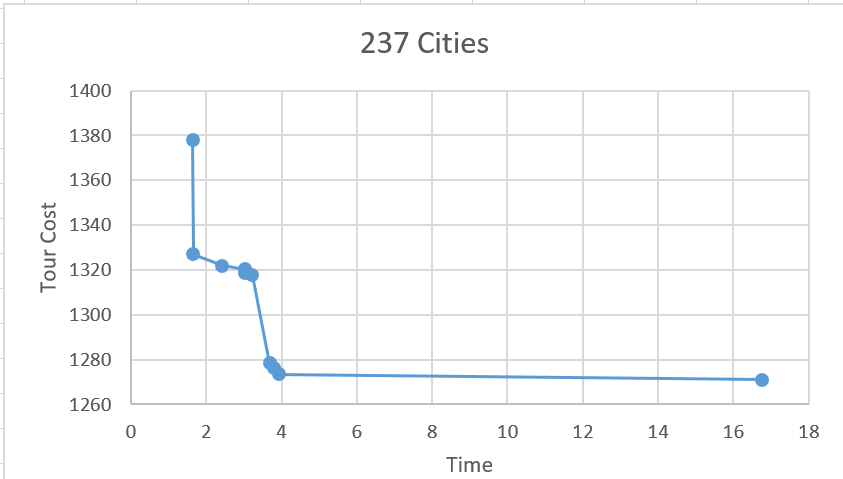
200 Cities isn’t too bad. That’s twice as many cities, and exponentially many more tours than the 137 city problem. Let’s try doubling again: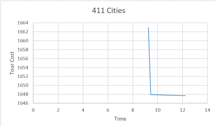
400 cities is twice as big again. Things are starting to get a little rough. It takes several seconds to find the first solution. Then we don’t find a new solution between 12 seconds and 5 minutes. Still, we were able to find some solutions to the problem. It’s just that we don’t love the way that the anytime search profile is shaped. Let’s throw in another 200 cities: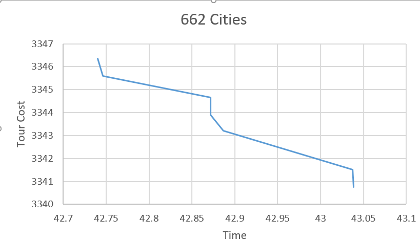
Now we aren’t finding solutions for nearly a minute. Then, we hit a large stream of solutions in the space of a second, then radio silence from the algorithm from many more minutes. There’s something about the search strategy that causes us to visit large pockets of solutions, then get stuck there for a long time. It’s the child ordering. A subtree in one of these search spaces tends to be pretty large. In the example above, before we consider pruning, every child of the root contains 661! possible tours. If we ask google calculator how big 661! is, it says infinity, which is not technically true, but it is pretty true practically speaking. That number is so large that we can never expect to visit the whole subtree of the first child of the root, let alone the 137th child of the room. If the optimal solution to our problem lies beneath the 138th child of the root, that’s a serious problem.
We know we our search algorithms can get stuck, but they do seem to find solutions to problems of decent size. Let’s ratchet it up to a crazy level and see what happens. I found a list of all 115,475 cities in the continental US to work with. Other than our patience, is there anything that stops us from tackling such a huge problem? Let’s run it and see:
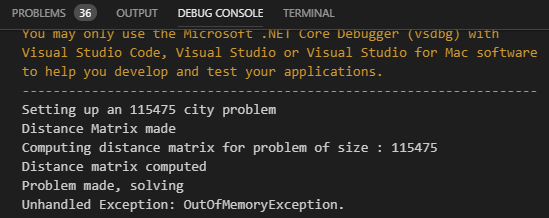
Well, we blew up all of memory. That’s not surprising; the distance matrix for a 115,475 city is pretty big. 115,475 * 115,475 / 8 gives us the number of bytes consumed by that distance matrix. Turns out, it’s a few terabytes, and I just don’t have that on my desktop. Even removing the distance matrix and computing distances on the fly won’t fix the problem; recall from line 8 of the TSP representation above, each state stores a boolean array recording every city that it’s visited. Any path through the tree is going to be exactly 115,475 cities long. The depth first search we implemented last time maintains a list of all viable children at every depth. So, at depth 0, we store a 115,475 bit array. At depth 1, we store 115,474 115,475 bit arrays, which is a little over a gig of memory. By depth 2 we’re consuming two and a half gigs, by depth 3 nearly 4 gigs of memory. The search tree uses too much memory in this representation.
Summary and Next Steps
We can solve some pretty big permutation problems using the search code we wrote last time. Remember, we didn’t actually implement anything new in terms of search in this post; we relied on entirely the same problem solving strategy for sorting pancakes and routing between shops to buy batter. That is one of the most powerful things about heuristic search. Beyond the power of general problem solving, we took a closer look at heuristics. We saw that there were two uses for heuristics: ordering the nodes in the tree for search and providing bounds on solution cost to aid in pruning. Finally, we talked about the fact that depth first search is an anytime algorithm, or more explicitly it is an algorithm which provides a stream of improving solutions. A stream of solutions is convenient, as it lets our algorithms work in situations where any solution fast is desirable as well as in situations where only the best solutions will do. Further, anytime algorithms can work in processes that fall anywhere between these two extremes!
What Are We Looking At Next Time
We ran in to two hard problems when running depth first search on really big TSP problems. One is that we didn’t have enough memory to solve really large problems. Even when we stripped down our problem representation, our state representations were too large to fit the search tree in memory. Next time, we’ll look at some clever tricks for reducing the memory footprint of the search algorithm. This will let us start to find solutions to that 115 thousand city problem.
The other problem was that our anytime search curves weren’t nice. Depth first search would find short bursts of improving solutions and then nothing for several minutes before emitting another short burst of improvement. This is because depth first search places too much value on child ordering, preventing it from seeing large portions of the tree for huge swaths of time. Next time, we’ll substantiate that bald assertion, and we’ll take an in depth look at what it really means and how much of a problem it can be. We’ll finally move on from depth first search and look at some techniques that spread search effort more evenly across the tree.
