
Last Time
Last time we took a look at how improved bounds computation and child ordering can improve the performance of heuristic search algorithms. In particular, we saw how those techniques improved the performance of depth first search (or depth first branch & bound if you prefer) when applied to the TSP. Even though we made a couple of improvements to the depth first search algorithm, we found ourselves unable to solve the really hairy problem we had our eye on: the 115k city TSP. We just kept running out of memory.
Learning Goals
This time around, we’re going to look at a technique for saving memory in tree-based search algorithms: the delta stack. Briefly, delta stacks allow us to keep track of a single state and the changes made to it, rather than a set of states when performing search. If the changes are small relative to the size of the state, this can be a huge savings.
Delta Stacks
Delta stacks are a fairly important technique for reducing the memory footprint of a tree-based search. There are lots of reasons you might care to reduce your memory consumption:
- Give yourself more space for memory based heuristics
- Give yourself more space for bloom tables for duplicate detection on graphs
- Reduce the cost of running the algorithm on a service like AWS or Digital Ocean
- A single path to solution is too big to fit into memory
We’re in that last category when we attempt to solve the 115,000 city TSP. We just don’t have enough memory to represent a single solution in memory. That sounds like an insurmountable task, but we’ll see that it isn’t.
Why does this work?
You may recall from previous posts that our first implementation of depth first search was too inefficient to solve any problems at all. This was because we blew up the call stack because we weren’t being careful about our recursive calls. Even when we fixed that, our search was pretty slow. This was in part because we were greedily generating all children during the search. This is what is shown in the image below. The search algorithm starts at the root and generates all of its children, throwing them on to the stack. Then it takes the first child from the stack, some child of the root, and generates all of its children. These grandchildren of the root are then thrown on the stack, and so on and so on, until we get the tree you see below.
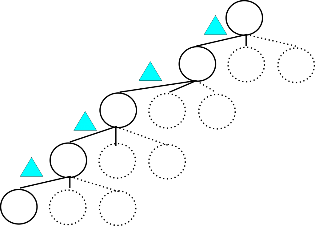
We then talked about how lazy child generation was key to getting a performant search algorithm. Lazy child generation just means that you generate the children only as they’re being considered by the search. We previously talked about how this is done: by keeping track of a child index so that we know which child is the ‘next’ child to generate. You can see the savings of such an approach below. The solid nodes represent the current avenue of search which must be held in memory, and the dotted lines and circles are for nodes which the search will generate later when it walks back up the tree to reconsider these potential solutions. They also exactly represent the savings realized by using lazy child generation.

Delta stacks as an extension of lazy child generation
Delta stacks are in some sense just the logical conclusion of this line of search optimization. The core of the idea is noticing that the difference between nodes in the search tree is generally quite small relative to the nodes themselves. For our current example, the traveling salesman problem, we change the following things when moving between two nodes in the tree:
- The number of cities we’ve visited is increased by 1
- The city we are currently at is changed
- The bool array showing where we’ve been is updated
So, that’s 1 bit and two integer updates for each state if we only talk about what needs to be changed. If we consider what needs to be generated, we still need to generate two integers: one for the city we’re in and one for the count of places we’ve been. However, we also need to construct a fresh bool array to keep track of exactly which cities we’ve visited. That’s an additional 115,000 bits that need to be allocated to make the new state. So, in this case, and many others, the state is far larger than the changes.
How?
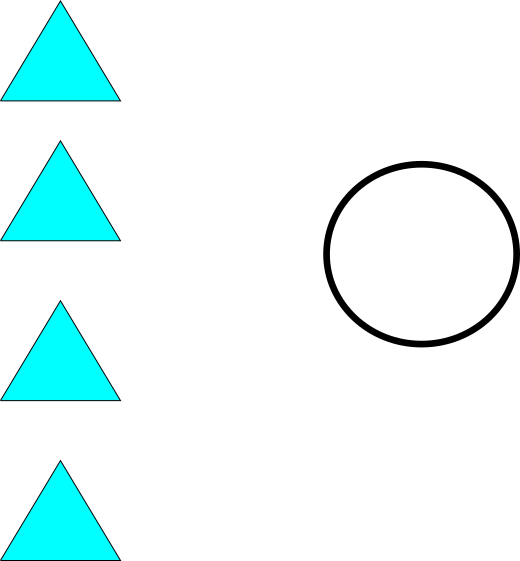
We can save ourselves some memory, and in some cases time, by keeping track of a single state and a stack of deltas telling us how we got there. The memory savings are hopefully obvious given the example from TSP above. If they aren’t, hopefully the image below will help clarify. This is an equivalent representation of the search tree above: four deltas and a single node. The deltas are smaller than the nodes, so we’re saving whatever the difference of four nodes and four deltas is in terms of memory consumption.
One way to think about this is that before the stack used by the search algorithm was a stack of states in the problem space. Now, we’re dealing with a stack of actions in the problem space. Applying or undoing the actions on the stack allows us to move from one state to the next and perform all of the common search actions:
- Heuristic computation
- Cycle Detection
- Goal Tests
- Pruning on incumbent solutions
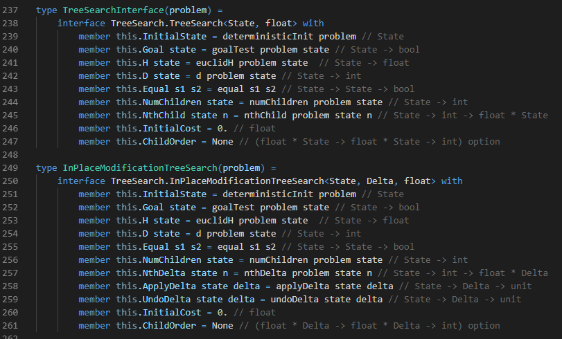
Below, we see the alterations that need to be made to the search interface in order to handle delta stacks. This approach is more commonly called ‘in-place modification’. It’s called that because we’re modifying a single node ‘in-place’ by applying and undoing the deltas.
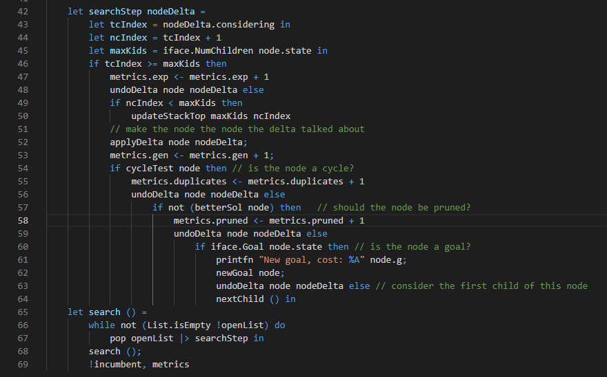
Of course, the search code also needs to change. We’re not dealing with states any more, but deltas. That is, we really are still dealing with states, but we get there by applying deltas and undoing deltas as the search progresses. There’s a little more book-keeping involved in our search algorithms now, but it isn’t too bad:
Impact
The difference is night and day; specifically, the difference is solving the problem at all or failing because of memory issues. It takes a little over half an hour to issue our first solution, and we don’t see another after that for several hours. This is because:
- Computing the pairwise distance matrix for 115,000 cities takes a while
- The initial solution is quite strong
- The search space is enormous (115,000! is real big)
Next Time
Obviously, the solving time we saw above for a single solution is unacceptable. Even if we wait a few hours for improving solutions, we don’t get very many. Next time, we’ll look at how to parallelize depth first search. We’re going to look at single machine, multiple core parallelism first. This will let us trade development and CPU time for some wall-clock time when we search for solutions to our problems. Then, we’ll look to move from single-machine parallelism to multiple-machine parallelism in the post after the next.
