Last Time
Previously, we looked at a technique for reducing the memory footprint of a heuristic search. We talked about why it was important to reduce the memory consumed by a search. Even if we move heaven and earth to reduce memory consumption, heuristic search is still prohibitively expensive in terms of time.
Learning Goals
This time, we’re going to look at reducing the wall-clock time needed to solve a search problem by using parallel computing. If you’ve not heard the term before, wall-clock time is exactly what it sounds like: how much time goes by according to the clock on the wall. In particular, we’re going to look at how to perform heuristic search in parallel using multiple cores. That is, we will look at how to use multiple processes in the same memory space to perform search quickly. This will set the stage for talking about distributed heuristic search, where we will use multiple computers to perform search quickly.
Parallel Depth First Search
First, a word on what parallel heuristic search is. As the name suggests, it’s where the search for solutions to the problem is performed in parallel. Depending on the type of heuristic search algorithm you have, you may find it trivial to parallelize, or you might find that task nearly impossible. Part of the reason that this series has been focusing on depth first search, a tree search algorithm, is because it parallelizes well. Let’s see why.
Why is it possible?
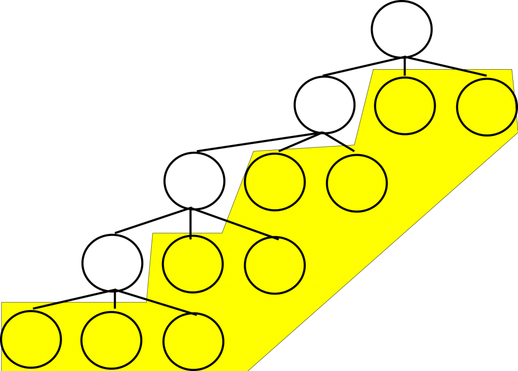
The image below should be familiar to us by now. It’s a caricature of depth first search exploring a search space for a problem. As before, the left child of the root is the most promising, then the second most left, and so on. Here, we’ve highlighted some nodes yellow, and some nodes white. Imagine for a moment that you’ve taken the root of the problem, the highest node in the tree that is in white, and expanded it’s best child, and the best child of that, and so on, four times. This is, more or less, exactly the way depth first search behaves: repeatedly expanding nodes beneath a root.
If you expanded nodes in the manner we described above, you would be left with the nine nodes we see below in yellow. As you may have noticed up to now, depth first search really doesn’t let branches interact with each other heavily. In fact, depth first search only really allows interaction between branches of the tree when we consider pruning on an incumbent solution to the search problem. This limited interaction on search branches lets the algorithm parallelize well. In fact it parallelizes trivially: we can treat each node in yellow as the root to its own search problem. This gives us, in this specific case, nine problems to solve in parallel.
The figure below further refines that notion. We’ve colored each of the nodes differently to show that each could run on its own processor. Each node, when solved, presents its own solution to the global problem. We then simply take the best solution from the ones found. Generally any depth first search algorithm can be parallelized by running it until the size of its stack of open nodes is equal to its budget in terms of concurrently running process. Once they are equal, you simply solve every node in the stack in parallel.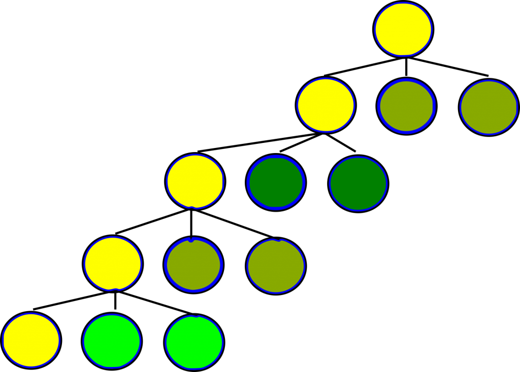
Why is it a good idea?
If you’re familiar with parallel computing, you might recognize the above as being a description of an embarrassingly parallel task. Depth first search requires little to no effort to separate the tasks. Here, task is literally “search beneath a given node”. Communication between tasks, or nodes in the search tree, in depth first search is limited to sharing cost of the incumbent solution, as we said before.
Unless you’re in a strange case where every node in your tree is a solution, there should be a pretty good work to communication ration for a give tree search problem. Said another way, solutions should be rare compared to other nodes in the tree. You might be so bold as to hope that we would see linear speedup, that is if we use N processors to solve the problem, we might see an N factor reduction in solving time. This can happen, but it’s even better than that. There are many domains in which parallelizing depth first search causes super-linear speedups. That is, for a processor budget of N, you see more than an N-fold speedup.
There’s a wealth of literature explaining how that can happen, but we won’t explain that in any detail. We will, however, see that for the case of N=2 we do see a super-linear speedup with the approach we take on some instances of the pancake problem. For now, we’re going to focus on how to parallelize the algorithm at all.
How do we do it? – Broad Strokes
Loosely, we do the work of searching the space in two segments. The first part of the work is simply for priming the parallel solving queue. We need to have enough nodes in our tree to hand one out to every processor that’s made available to us. After this priming step, each processor will be handed a node somewhere in the middle of the tree to treat as the root of its own search problem. Each worker will independently search that space for solutions and report back.
Executor Talks to Workers
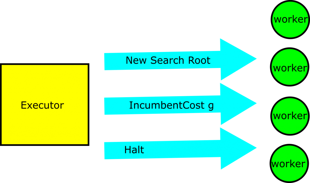
We’ll refer to the program that preforms the priming step and distributes work to other processes as the executor. All other processes will be called worker processes. I find that one way to understand a parallel computing process is to think about it in terms of how the elements communicate with one another. Below, we see the communications that can occur between the executor and any working node:
- New Search Root- the executor hands a new problem to the worker for it to solve
- IncumbentCost g – The executor tells the worker that the best known solution to the problem has cost g, and that the worker shouldn’t bother exploring paths that don’t improve on that
- Halt – Stop everything you’re doing, we think the problem is solved or someone has told us to stop running.
Communique 1 is how we tell a worker to start solving a part of the problem for the overall distributed system. In the process we’ve described above, we’ll only see one such message, during the start up phase of the parallel computation. Communique 3 is just there for gracefully stopping the parallel program. It’s Communique 2 that does half of the coordination of our paralell processing efforts. When the executor learns of a new solution to the problem (we’ll see how this happens below), it communicates the new bounds out to each of the workers. As we saw in a previous post, effective pruning has a huge impact on depth first search performance. Therefore, it’s critical that we send this message out to each of the workers as soon as we can.
Worker Talks to Executor
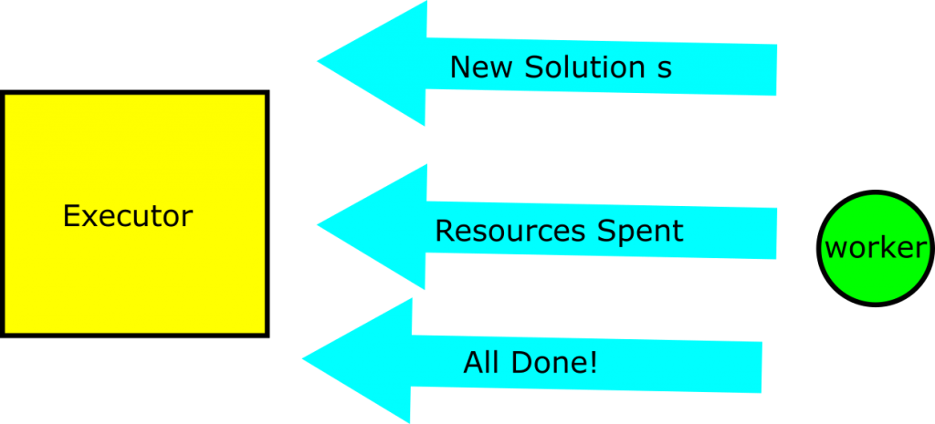
The following are the three kinds of message that an individual worker can send to the executor:
- New Solution S – I’ve solved the problem, here is the solution and its properties (including cost).
- I’ve spent this much trying to solve the problem so far
- I’ve exhausted the tree that you handed me, and I am done executing.
Communiques 2 and 3 are for figuring out how ‘expensive’ it was to solve the problem overall in terms of compute resources; said another way, they’re for book keeping. Communique 1 is the coordinating message. It tells the executor, and by extension all of the other workers, that a new solution has been found. The executor then pulls out the new solution cost, and tells all of the other workers about the new incumbent solution cost.
Wait, why aren’t the workers just talking to each other?
There’s one obvious reason you might want the workers to talk to each other rather than the executor: the executor looks a lot like a bottle neck in the communications here. That’s true, but remember that its only job is coordinating the processes we’ve forked off. Additionally, it provides an important filtering function, as we’ll discuss next. Before we talk about the filtering though, there’s another reason you don’t want to have to make the workers talk to each other : they’d spend a bunch of time talking when they should be working. What we’re kind of enforcing here is a division of concerns. The workers search and the executor coordinates.
I said the executor acts as a filter. Specifically, what it filters is non-improving solutions. In previous iterations of depth first search, it was impossible to produce a non-improving solution because of how we pruned on the incumbent solution during the search. However, with a parallel approach comes some communication overhead. When a worker finds a solution, it must tell all of the other workers.
Even if we were doing this directly, it would be possible for thousands of nodes to be generated between finding the solution and sharing its cost with our peers. During that time, other solutions might be found. These could be just as good, or they could be better. By passing all of the solution messages through the executor, we can make sure that the worker nodes only see a stream of improving solutions for pruning. Similarly, we can present a stream of improving solutions to the user, even if that isn’t strictly speaking what we find.
How do we do it? – Specifically
When I approach a distributed system, I start by thinking about how it communicates. We realize the communiques in broad strokes above in F# below. We split messages into two categories: MessageToWorker and MessageToExecutor. These, as the names hopefully imply, are messages to the workers and to the executor respectively.
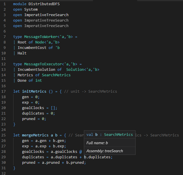
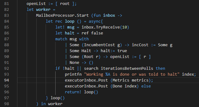
In a vacuum, these messages are not particularly interesting; however, their use is interesting. Below is code for the core of the worker’s process. A worker processes mailboxes, as we see on line 82 and 83. This is just a way of saying that it’s an asynchronous processes that handles some messages in a queue. It processes the MessageToWorker messages defined above.
Changes to Search for Worker
The worker proceeds as follows: on line 85, it sees if it has any message to process. If it does, it handles it in the match case starting on line 87. A new incumbent solution causes it to update the bound on solution cost in line 88. Line 89 is how we start the worker process on a new node; the stack of all nodes to explore for the worker is initialized to be the singleton list of the root. Line 92 is where the bulk of the work is done. So long as we haven’t been told to halt, search for a certain number of iterations between polling your message queue. To drive that home, we changed the following things about the search:
- We added some functions to send messages about 1. New solutions
- Resources Consumed
- Exhausting the space
- We search for a fixed number of iterations between polling an inbox
We could take more complicated approaches to parallelism to avoid the gating and the polling done here, but we don’t have to in order to improve performance and take advantage of additional resources as we’ll see below.
The Newly Minted Executor
Whereas the worker is search at its core, the executor is new. That’s largely because it’s not doing search so much as it is coordinating several search processes. Message processing happens on lines 119 to 127. Here we’re looking for nodes announcing they’ve completed all of their work (line 127), reporting how many resources they consumed over all (line 126), or telling us about a new incumbent solution (line 122). It’s this case that is interesting. When a new incumbent is found, we check to see if it is better than the best solution we know about (line 124) and then if it is we communicate it to all of the workers (line 125).
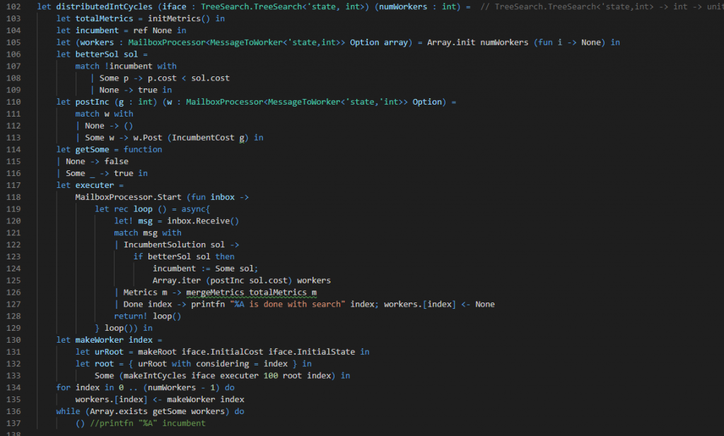
The other interesting thing the executor does is kick off several processes to solve the search in tandem. We supply the executor with its processor budget as an argument on line 102. The definition of worker construction begins on line 130 and ends on 133. Lines 134 and 135 actually instantiate all of the workers.
We use a particularly naive strategy to handle parallelism here. We hand each node a particular child of the root. If we have more processes than there are children of the root, the workers would stop immediately. This prevents us from scaling up arbitrarily. While this approach isn’t general, we were trying to solve a 115,000 city TSP problem, and I’m pretty sure my desktop doesn’t have more than about 8 cores for me to use. Given the huge difference in possible roots to hand these workers and the number of workers I can reasonably have on my desktop, we could have looked at interesting ways of selecting roots or spacing the roots evenly. That’s omitted for now because I want the parallelism to be as simple, and hopefully as understandable, as possible.
Finally, on lines 136 and 137, we see the overall coordination of the workers through the executor. The executor runs up until all of the workers have finished. It doesn’t do anything other than process messages in that time. Whenever a worker finishes, its entry in the array of all workers is changed from Some Worker to None (line 127). So long as some worker exists, Array.exists getSome will return true on line 136. Once all workers have finished, the executor is free to finish as well.
How does it change performance?
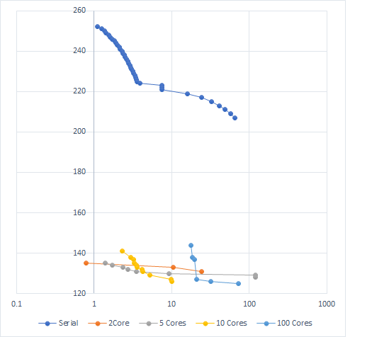
The above graph shows algorithm performance based on number of workers used. The Y-axis shows solution cost on a single instance of the 100 pancake problem. The x-axis reports time in seconds on a log scale. We take a look at the performance of depth first search when run with 1 worker (e.g. the serial case), two workers, five workers, ten workers, and one hundred workers. The line way up top on its own is serial performance. All of the lower lines are for the algorithm running in parallel to some extent. Here are some highlights from the results:
- All multi-core solutions are far and away cheaper than the cheapest solution found by serial search
- Two core search finds its first solution before serial search finds any solution – It is in fact more than twice as fast to reach the first solution.
- As you increase the number of workers used, time to first solution tends to increase – 100 workers is totally dominated by 10 workers
- There are 16 cores on the machine I’m working with, so that’s probably related.
What’s this mean? What’s next?
What I take away from this is that our distributed implementation of depth first search works decently. That’s good, because it’s a simple implementation without many of the bells and whistles you see of distributed search algorithms in the literature. That said, we’re limited by the number of physical cores on the machine we’re using. That’s bad. We’d like to be able to scale arbitrarily to take advantage of as much computing power as we can afford. Next time, I’ll talk about how we can take advantage of cloud computing resources to do the same thing we just did, but on lots and lots of computers at once.
Build awesome things for fun.
Check out our current openings for your chance to make awesome things with creative, curious people.
You Might Also Like
