
Heuristic search is a subfield of artificial intelligence. It is the study of algorithms meant for general problem solving. The problems solved with heuristic search come from a variety of domains, including:
- Aligning genetic sequences
- Planning routes between two cities
- Scheduling elevators in a building
- Scheduling work orders in a machine shop
These varried domains have two things in common. First, the difficulty of solving these problems grows far faster than the size of the problem. These problems are intractable. Second, these problems are representable in a common way:
- There are states, or configurations of the problem world
- There are actions, which change one state into another
- There is one, or a set of, goal configurations that solve the problem
Heuristic search is an active area of research, and has been since at least the 1960s. I spent the better part of my twenties thinking about heuristic search algorithms. I can, and would love to, talk your proverbial ear off about the subject of my research.
Instead, I’m going to focus on a more important aspect of my work than the new algorithms I developed: algorithm visualizations. At the time, I viewed the building visualizations as something that took me away from my primary research focus. That was wrong. Those visualizations helped me build a deeper understanding of the behavior of algorithms.
There are two kinds of visualization I used throughout my research. The first is the humble x-y plot of algorithm performance. The second were visualizations of algorithm behavior on grid pathfinding problems. The former identifies gaps between observed behavior and theoretical limits, fertile ground for new techniques. The later was useful for diagnosing and correct bad behavior in existing algorithms.
Understanding Exploitable Gaps In Bounds
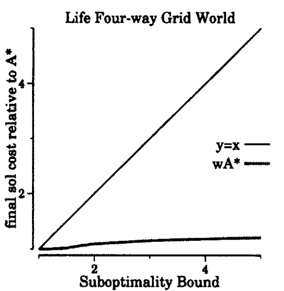
This graph shows the behavior of an algorithm called weighted A* on a grid pathfinding problem. The x-axis show how much more a solution returned by weighted A* can cost, relative to optimal. The y-axis shows how much more the solution returned by weighted A* actually costs. The line y=x shows the theoretical limit; weighted A*’s line must remain below here.
The important thing to notice about that line is the gap between y=x and weighted A* performance. Weighted A* often returns a solution much better than the bound suggests. This gap, between guarantee and actual, can be exploited to improve performance.
That’s exactly what we did in 2008, when we developed optimistic search. Optimistic search is a two phased search algorithm. In the first phase, it runs weighted A*, using a more generous W than the desired bound. In the second phase, it proves that the solution found in the first phase is within a much tighter bound.
The intuition provided by the first graph lead to the creation of optimistic search. There are other sources the same insight could have come from. For example, the gap is also present in the proof of weighted A*’s bounded suboptimality. That isn’t how it happened though. The visual gap in the graph is stark. Further, it relates to a parameter supplied to the algorithm. The plot makes it easy to notice that W can be significantly increased without impacting solution cost. Once you’ve made that observation, the optimistic search approach becomes obvious.
Understanding Bad Behavior and Correcting It
Prior work is a hugely important thing in academic fields. After presenting on optimisitic search, I was asked why I hadn’t compared against A* epsilon. The truth was that I had; those comparisons were in the paper. The behavior of A* epsilon was so poor that I didn’t include it in my presentation deck. In part because I didn’t want it to get in the way of my point. In other part, because we didn’t understand its poor behavior.
Not understanding prior work is frustrating for an academic. You’re meant to be building upon the work that others have done. You can’t do that unless you start by understanding what’s come before.
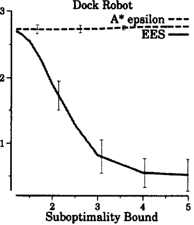
The thing that doesn’t make sense about A* epsilon’s behavior is that it gets worse as the bound is relaxed. At least, it does initially, as we see in the graph above. Bounded suboptimal algorithms are supposed to improve with relaxed bounds. We’d seen these sorts of problems before, and they were generally a result of revisiting nodes in a search problem.
Deeper inspection revealed that, indeed, A* epsilon reopened nodes frequently. We still didn’t understand why though. Knowing something is a problem isn’t enough to fix it. You have to understand the nature of the problem before you can address it. To understand the nature of the problem, we began visualizing the algorithm’s behavior.
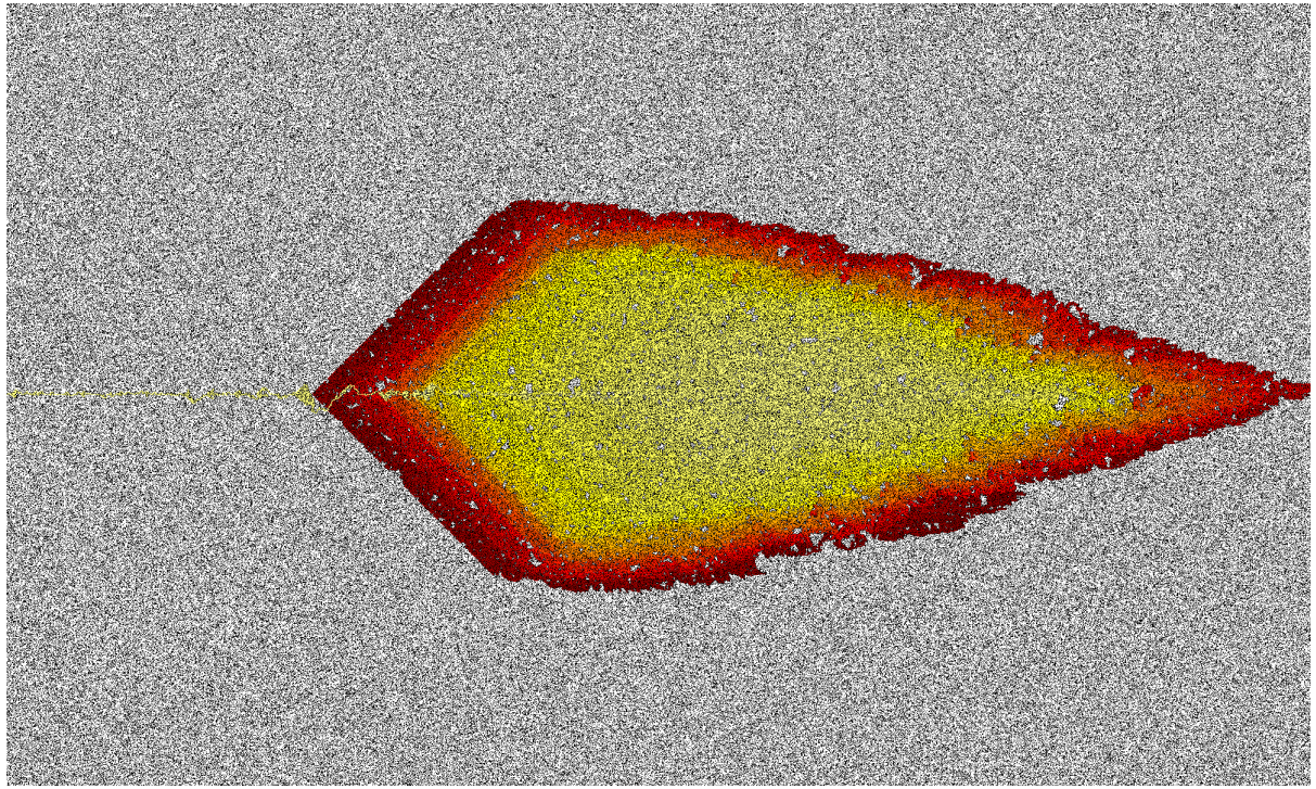
The above image shows a grid navigation problem solved by A* epsilon. The goal is to navigate across the image from center left to center right. Black cells are obstacles, and white cells are empty space. The colors from yellow to red represent A* epsilon’s expansion order. A* epsilon visits yellow cells early on in the search, while red cells are visited much later.
This image differs noticably from similar images from other search algorithms. Most striking is how A* epsilon spends the bulk of its search effort near the goal of the space (center right). Most algorithms spend the bulk of their search effort near the start of the problem (center left).
A* epsilon does exactly what it’s designed to do. It prefers to explore sufficing solutions that are as near to completion as possible. Generally, this sounds exactly like what a bounded search algorithm should do. It has bad behavior because proving a bound requires search effort near the start of the problem. A* epsilon avoids this and suffers from bad performance.
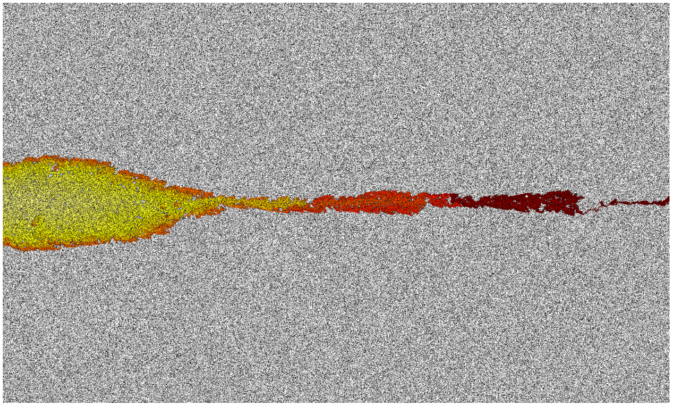
These insights led to the development of explicit estimation search, (EES) shown above. EES is like A* epsilon, but it has addilitonal rules that force it to consider nodes near the beginning of the search space where appropriate. Adding in this rule fixed some of the worst behaviors of A* epsilon. For a time, EES was the state of the art in bounded suboptimal search. We could only have gotten there by understanding when A* epsilon failed. We wouldn’t have understood the problems with A* epsilon without the visualizations above.
Conclusion
I spent the better part of my twenties thinking about heuristic search algorithms. Day in and day out, I labored to find new approaches that would improve on the current state of the art. At the time, I viewed the building visualizations as something that took me away from my primary research focus. That was wrong. Those visualizations helped me build a deeper understanding of the behavior of algorithms. Without that understanding, I couldn’t have built the techniques that were the backbone of my thesis.
