Introduction
Machine learning is at least as old as Arthur Samuel’s attempts to improve his checkers playing programs back in the 1950s (Some Studies in Machine Learning Using the Game of Checkers), if not older still. Despite being around for decades, machine learning has received intense interest recently from the public, the scientific community, and industry. This may in part be because machine learning has matured in two key respects: techniques have become more robust and effective. Additionally, many well developed libraries and products make machine learning more approachable than it has ever been. This presents a clear opportunity and need for software contracting companies. When a prospective client comes to us and asks “I have piles of information, what can I do with it?” or “I need to improve the behavior of the following system, can machine learning help?” we need to have a response. It would be even better if we had one backed up by successful deployments.
As a company we felt it important to have a compelling story about machine learning banked against a future need; therefore we decided to invest internally on experimenting with large in-house corpora to gain some non-theoretical experience and potentially improve some of the things we already offer to clients. The first, and often the most difficult, task is to identify to problems where machine learning is a good approach. Modern ML techniques are capable of learning complicated things. Further, we have many techniques to deal with data that are not meticulously curated. Even with their newfound power and robustness, machine learning is only very good at a small variety of tasks. One of these is separating things into one of several classes. Luckily, we had a very straightforward classification problem in house: given a series of data describing the performance of a turbine engine, decide what sort, if any, of problem it is encountering.
In the remainder of this article, we’ll look at how we used machine learning to approach this classification problem. First, we describe how we set up the data for use in supervised learning. Then, we’ll describe the system we set up for learning and evaluation, including the libraries we relied on for machine learning. Finally, we’ll look at some results from our evaluation of the machine learning algorithms. To give away the results, we found that, relying on only the data we had available along with classifications provided by an expert, we were able to correctly identify roughly 95% of engine problems.
Problem Description
We said that identifying issues with turbine engines from data describing its performance was a straightforward example of a classification problem; however, we didn’t explain what issues we were identifying, what a classification problem was, or provide any justification for that statement. We’re going to go back and fill in those blanks in the following paragraphs. We’ll start by describing how EHMS is used to identify issues in engines from performance data today. Then, we’ll talk a bit about what a classification problem is and how supervised learning can be used to solve it. Then we’ll see how we can use EHMS to train supervised learning algorithms to recognize potential issues in engine performance.
EHMS System for Identifying Issues in Turbine Engines
EHMS expands into the “Engine Health Monitoring System”, and it does exactly what’s on the tin. It’s a system for monitoring engine health. More directly, it’s a system for recording measurements related to engine performance over a long period of time. These measurements are associated with an engine, an airplane, and the position of that engine on that airplane. Then, the data are examined by a human analyst. They take a look at the performance of a particular engine or several engines over time. Looking at the trend of engine performance over time allows the expert to identify a wide variety of problems with the engine. Once identified, the potential issue is entered back into the system to let maintenance staff know that an engine is suffering from degraded performance, needs maintenance, and that the likely cause is the issue identified by the expert. Maintenance then addresses problems with the engine and additionally notes whether or not the original diagnosis from the expert was accurate. In addition to performance trend presentation for expert analysis, EHMS has a variety of other aspects which support fleet maintenance and readiness, but these aren’t relevant for the machine learning discussion here.
What is a Classification Problem? What is Supervised Learning?
Per wikipedia, a classification problem “… is the problem of identifying to which of a set of categories (sub-populations) a new observation belongs, on the basis of a training set of data containing observations (or instances) whose category membership is known.”. Less cryptically, a classification problem is the problem of assigning a class to a given thing. We teach an algorithm to assign the correct class to a particular thing by showing it lots and lots of examples of things along with their associated class. After seeing many examples, machine learning algorithms learn how to discriminate between different classes somehow, where the how differs by machine learning algorithm.
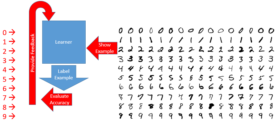
The above image is a rough diagram of how machine learning approaches the problem of classification. In that specific example, it’s a picture of how digit recognition works on the MNIST dataset. On the right of the image we have a large number of examples, segregated by class. On the left of the image, in red, we have the correct class labels called out for each row. This is what makes digit recognition a supervised learning task: we have labeled training data provided by an expert. You can think of the algorithm consisting of both a learner, which attempts to learn to perform some task, and a critic or supervisor which provides feedback to the learner so that they can improve their performance. The rough approach of the machine learning algorithms considered here is shown in the center:
- Present an example to the learner
- Have the learner produce a class for the example
- Evaluate the accuracy of the learner’s classification
- Provide feedback to the learner
Learning algorithms differ in many ways, including how they consume feedback and whether or not they train on a single instance at a time (online learning) or if they consume all of the training set upfront (batch learning). You can always feed batch data to an online learner by iterating through the elements of the batch and feeding them in one at a time. We used both kinds of algorithms, that is batch and online, in our evaluation below.
How do we turn EHMS Issue Identification into a Supervised Learning Problem?
Having discussed how EHMS is used and what the basic components of a classification as a supervised learning problem, we will look at how we turned engine issue identification into a classification problem. We address this in three steps. First, how did we find labels for the supervised learning problem. Second, what data are available for machine learning? Finally, which data did we give to our learning algorithms and why?
Getting the Class Labels
Central to the notion of a classification problem are identifying the available classes and finding a correct mapping of instances to classes. The first defines the problem itself, while the second allows us to apply and evaluate supervised learning algorithms to the classification problem. In the case of EHMS, one obvious set of classes are those provided by the ‘likely cause’ value for engines identified as being in need of maintenance or closer observation. There are 19 such labels, and they include things like unbalanced props on the airplane and sensors being out of alignment. Critically, that set of labels doesn’t directly include a label for instances where everything is ok. For this dataset, we assume that if the expert hasn’t identified an issue with an engine that they are declaring that there is no issue with the engine. This way, we end up with 20 total classes, 19 of which identify various problems with the engines, and 1 for engines that are operating correctly.
It isn’t enough to simply have a set of classes for supervised learning of classification. You also need to know that those labels are correct, and further you need to be able to associate the labels to data for purposes of classifying the data points. To the first point, we have feedback from the maintenance crew to determine if the expert applied label was accurate. Specifically, when performing maintenance tasks, the mechanic enters whether or not the maintenance dictated by the likely cause provided by the expert was effective, not, or of indeterminate efficacy. For our purposes, we consider those instances, and only those instances, where the mechanic says that the dictated course of action was effective to be examples of properly applied labels. In the case of the “everything ok” label, we only consider those to be accurate if the engine in question has yet to be removed for any variety of maintenance. That addresses the correctness of the labels. Association of the labels to the data we use for training is achieved by relying on unique identifiers for engines, aircraft, and the installation position of the engine on the aircraft which are stored both for analyst alerts, maintenance reports, and any flight data dumped from the plane after a flight.
Selecting Features to Learn From
Labeled instances is only half of the supervised learning equation; you also need a features to learn against. Features is just a succinct way of saying “properties of a thing which can be measured.” In the digit recognition example above, these features are the intensity of pixels, formed into an array. For our engine issue identification problem, we have an array of measurements relating to turbine engine performance during takeoff and cruise. The array contains around 150 elements for each datapoint we’d like to apply a label to. 150 may sound like a large number, but in practice it’s not a problem for the machine learning algorithms used here in terms of the size of the input.
While the size of the vector isn’t problematic, unfortunately its contents were; some features are, more or less, repeated. For example each vector contains raw measurements from sensors, rolling averages of changes between sensor readings, and absolute values on those rolling averages. This effectively rolls the same information into our vector three times. While including data multiple times in the feature vector isn’t catastrophic, it can cause some features that aren’t repeated, or aren’t repeated as often, to be discounted. If the features being drowned out are important for learning the target concept, then you might see poor learner performance as a result.
The solution is easily stated but difficult to execute: select a subset of the entire available feature vector to make the learning work better. We used two techniques that helped us settle on a final feature vector for our learners. First, we thought real hard about the features in the vector and which might were likely highly correlated to one another just based on the meaning of the feature. You could do this with statistical analysis, but since elements of our feature vector had names and descriptions associated with them, it was faster to think about what they contained and whether the described dependencies constituted a repetition. The second tool we used was empirical evaluation; we tried dozens of subsets of the features and evaluated the accuracy of the learning algorithms using those subsets. In effect, we used the machinery we built to train one supervised learning algorithm for classification to train hundreds, then we compared their performance and selected the best ones. We’ll talk about that machinery next.
Approach
Our General Approach
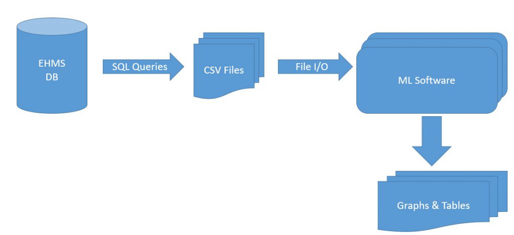
The general approach we took to training machine learning algorithms on the EHMS data is shown above. We start by extracting labels and data vectors from the database that backs EHMS via a set of SQL queries. The data that we get from these queries are dumped to comma separated volumes and stored for later consumption. The files are ingested into a python program which aligns the labels and feature vectors such that we have a large set of labeled instances to work with. The labeled instances are shuffled, and a prefix of the list of instances is reserved for testing. The remaining instances are used for training. Training instances are fed to each of the learning algorithms. Once training is complete, the test set is used to evaluate the performance of each of the learning algorithms. This evaluation is presented to the user in the form of graphs and tables of key values.
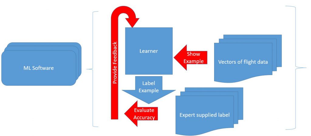
The figure above drills in to the machine learning portion of our general pipeline above. The approach is practically identical to that of the digit recognizer shown above. Where we differ are our inputs. Rather than vectors of pixel intensities, we use vectors of flight data. Similarly, rather than digit labels, we use numeric labels representing identified issues with engines. The general machinery of learning is unchanged, even though the setting is drastically different. That’s the power of machine learning; once you understand the setup for a particular application of machine learning, moving between domains for a given application is relatively simple.
Libraries Used
- Scikit-learn – machine learning toolkit for python
- Matplotlib – generating graphs for evaluation
- Scipy – Large data set manipulation and scientific computing tools
Above we provide a list of the libraries used in our implementation. We had libraries that implemented the machine learning algorithms, as well as libraries for the evaluation we performed on those algorithms. It’s worth mentioning these libraries because we didn’t have to implement any of what might be considered ‘the hard parts’ of machine learning for our evaluation. The bulk of the python we had to write for our learning and evaluation was for reading data out of files and putting it into the proper format for the learners to consume.
Evaluation
An important part of our pipeline was evaluating the performance of machine learning algorithms. It was important because it allowed us to tune our selection of algorithms and features in order to get the best performance of a learner on our dataset. As we’ve alluded to previously, training a classifier isn’t the end-goal of machine learning. You want to use the learned algorithm to do something, like automate a previously manual task, or improve human accuracy and throughput for a particularly complicated operation. Getting a learner that performs well is critical, but it isn’t the end of the story.
In order to evaluate the performance of the learner, we split our data into two sets: the training set and the test set. The training set is used to teach the learners the target concept. The test set is used to evaluate how well the learners did at learning the concept in question. Evaluation can be performed in a number of different ways, but the general idea is that you compare the output of the learner to the known correct label. You do that for each learner for each instance in the test set, and you aggregate those results to build a plot or a distribution from which you can infer more significant conclusion. We performed three such evaluations: comparing learners to the expert in the event that we know the expert is correct, comparing learners to expert in the event that we know the expert is wrong, and evaluating the learner on instances where the expert has not yet identified an issue.
True Positives
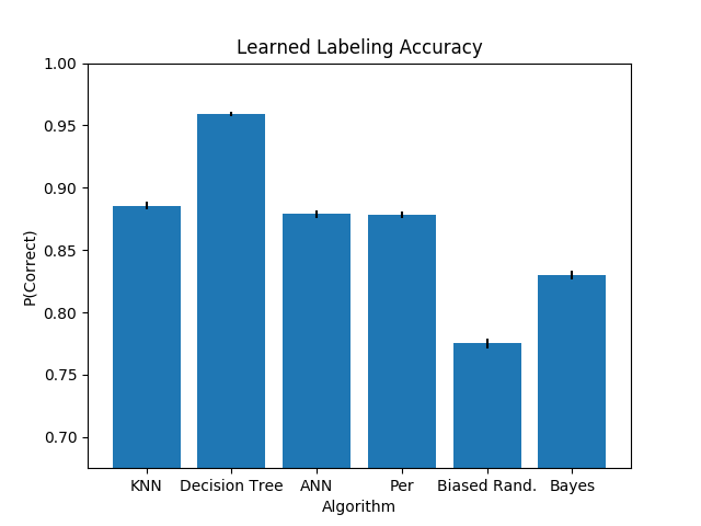
The above plot shows the performance of various learning algorithms when compared to that of the expert for true positives. A true positive is when the expert places a label on a given engine, say that the prop is out of balance, and we can confirm through other means that the problem causing the trend that they saw was exactly that the prop was out of balance. Generally this means that a mechanic performed whatever maintenance action is recommended to correct the issue identified by the expert, and the mechanic then confirms that the suggested fix was effective. The comparison here tells us how often the learners agreed with the expert, specifically restricted to the cases where the expert could be shown to be correct.
More specifically, bars in the plot above are generated as follows: Each learner is presented with the data in the training set and the attendant labels. It uses these data to learn. After learning is completed, it is presented with the examples in the test set in sequence. For each learner and for each example in the test set, we present the vector of features to the learner and compare the label it produces with the known correct label. If the label produced by the learning algorithm and the label known to be true are the same, we award the learner a score of 1. Otherwise the learner is awarded no points for that instance. This is repeated for all learner sand all test instances until we have a large collections of scores for each learner. The score is, roughly, the probability that we would expect the learning algorithm and the expert to agree on a given instance, with a score of 1 being “correct all of the time” and a score of 0 being “always wrong”. The bars in the chart show the arithmetic mean of the scores collected, while the black nubs on the top of the bar show the 95% confidence interval about the true arithmetic mean.
When looking at the chart, we can see that decision trees have the best performance of all learning algorithms considered in the evaluation. They’re between 96 and 97% accurate to the expert, meaning that for labels from the expert that we considered to be correct, they agreed with the expert labeling a little more than 96% of the time. This is a substantial improvement over other algorithms considered (about 8%). There’s a large amount of separation between 95% confidence intervals about the performance of decision trees and the 95% confidence intervals of all other learners. This means we can be very confident that the difference in performance is meaningful, rather than just a fluke of the random division of the set of labeled instances into training and test sets.
False Positives
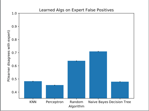
True positives aren’t a complete view into the performance of an expert or a learning algorithm. The above plot is meant to help complete our view by considering how the learners perform on instances where we think the expert mislabeled the example. These are specifically instances where the expert applies a label to an engine, the mechanics go out to perform the suggested maintenance, and find that this does not improve the performance of the engine as expect. In these cases, we suspect that the expert has made a mistake in labeling the likely cause of the engine’s degraded performance.
As before, each learner is presented with a set of instances for training and a different set for evaluation. As before, the training set is composed exactly of those instances for which we are certain that the expert was correct. However, the test set and evaluation criteria change. The test set is composed entirely of instances which we believe that the expert got wrong, per the mechanics feedback. Instead of assigning a score of 1 when the learner and the expert agree, we assign a score of 1 whenever the learner and the expert disagree. So, to be clear, we aren’t measuring how often the learner is right and the expert is wrong, we’re measuring how unlikely is the learner to make exactly the same mistake as the expert.
In the plot, we see that the naive bayesian classifier is least likely to make the same mistakes as the expert which sounds promising. However, recall that the overall accuracy of naive bayes was not good. It performed worst of all learning algorithms considered. When we restrict our consideration to the best performing learners in the true positive case, we get a different perspective. Each algorithm that did well tends to disagree with the expert about half the time in the cases where the expert is wrong; however, this is less than the weighted random approach, which disagrees with the expert about 70% of the time. Since the learns in question all perform ‘worse’ than the random baseline on this metric, we know that we’re learning to make the same kinds of mistakes that the expert did. That we don’t score 0 is encouraging, of course, but we’d like to do better than a weighted coin flip.
Unlabeled Instances
Not all instances, meaning not all traces of records coming from an engine on a plane, are labeled by the expert. Generally, we expect that means that there was no issue with the engine. In fact, we use those instances as examples of true-positive “everything’s ok” during training. But what if we entertain for a moment that those instances aren’t OK, but rather that the expert has yet to identify what the issue is? That’s what we do in the following evaluation. As before, we train on instances that are labeled by the expert and confirmed by maintenance on the engine. However, for the set of instances we evaluate post-training, we restricted ourselves to engines which were currently deployed for which the expert had yet to identify any potential problems.
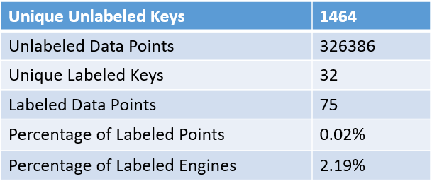
The above table summaries some interesting statistics about the test set and the performance of the learner (we only evaluated using decision trees here) on that set of data. There were around 1500 uniquely identified engines deployed. We had over 325,000 data points spanning those engines. The learner identified fewer than 0.02% of all data points that might be problematic, which corresponds to about 2% of all engines. For each of the 32 identified engines, we took a look at the performance trends of those engines, using the same criteria that the expert used to identify problems within EHMS. An example of these trend plots are shown below.
We wanted to see whether the labels applied by the learner were plausible. In the cases where the labels seemed plausible, which was most, we asked the expert to follow up for us, as their labels were going to be more accurate and not biased by a desire to see the learning algorithms perform well. In the cases examined, we didn’t always recognize the correct issue, but would frequently mistake two related issues (e.g. a general loss of pressure in the engine would be identified as having a specific, but rare, root cause rather than the applying the correct but more generic label). This was at the same time both disheartening and comforting. Ideally, you’d get the correct label on every instance considered. However, if you’re going to make a mistake it’s nice to at least be in the neighborhood of the correct answer.
Conclusions and Future Directions
How did we do?
Overall, the results of applying machine learning to classifying potential issues with engines from data to EHMS was relatively successful. We have accuracy like that of the expert, as we saw in the true positive evaluation. We avoid making some of the same mistakes as the expert, as we saw in the false positive evaluation. However, the evaluation on the unlabeled instances shows us that we don’t achieve the kind of accuracy that you might want for a wholly automated deployment. That is, we get in the neighborhood of the correct answer, but we aren’t exactly accurate. What we have is something that would be very appropriate for augmenting the capabilities of the experts analyzing EHMS data. Our machine learning algorithms could be used to triage engines for examination by ranking the severity of the labels applied by machine learning. We could potentially improve throughput by suggesting issues for each engine and having the expert verify them or supply their own alternate labeling.
What should we try next?
Going forward, it might be interesting to break the classification problem up into a series of classification problems based on an expert supplied taxonomy. From the limited number of examples we’ve investigated by hand, it seems to be the case that when we’re wrong, we still manage to be in the neighborhood of the correct labeling without getting the exact label correct. To use a more biological analogy, we manage to identify the genus but not the species. If that’s actually a general trend for our learners, then we could probably improve performance by training several classifiers and applying them in series: First, we’d train a classifier to recognize the general category of issue the engine is suffering. Then, we’d train a different classifier for each general category to recognize the specific issues within those categories. There are two general ideas at work here: learning algorithms tend to treat all mistakes as being equal, and the larger the number of classes one needs to recognize, the harder it is to train an accurate classifier. By setting up a taxonomy of issues for engines, we reduce the number of classes that we need to be able to discriminate at each level of the taxonomy. Layering the decisions lets us more accurately report the notion of ‘near misses’ in classification for an empirical evaluation, and reducing the size of the set at each level should theoretically let us train more accurate recognizers.
